Forecasting population, forest area and food production of World countries using an R Dashboard
Sulekha Aloorravi
Dashboard Link - Shiny Apps:
https://tinkleolive.shinyapps.io/rapp/
HTML Link - Github:
https://sulekhaaloorravi.github.io/ShinyDashboard/
R code in Github:
https://github.com/sulekhaaloorravi/ShinyDashboard/tree/master/code
Frame - Problem Statement
- What would be the population of various countries in the world until 2023?
- What Food quantity would we require to produce until 2023?
- What will be the Forest area and Agricultural area until 2023?
- How much food would be wasted until 2023?
- Forecast these data in an interactive graphical dashboard.
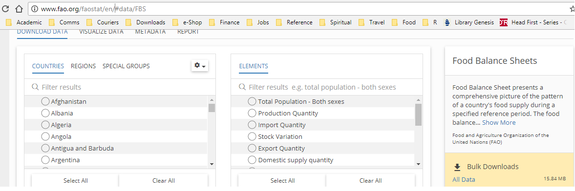
Acquire data
Data is acquired from Food and Agricultural Organization’s website FAO
Data downloaded was in zip format and it was further extracted into csv.
Refine
Downloaded data had to be refined since its struture was completely unusable for this analysis. Extracted zip file was exceeding 1 GB and it required a lot of
normalization to be done before using it in R. So I used an SQL database to normalize this data and convert it into R friendly csv data that can be read into a
dataframe.
Downloaded data 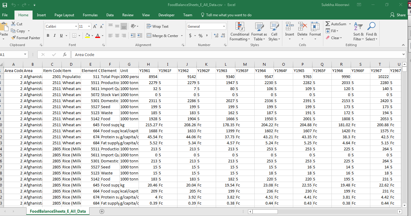
SQLite Database for FAO data 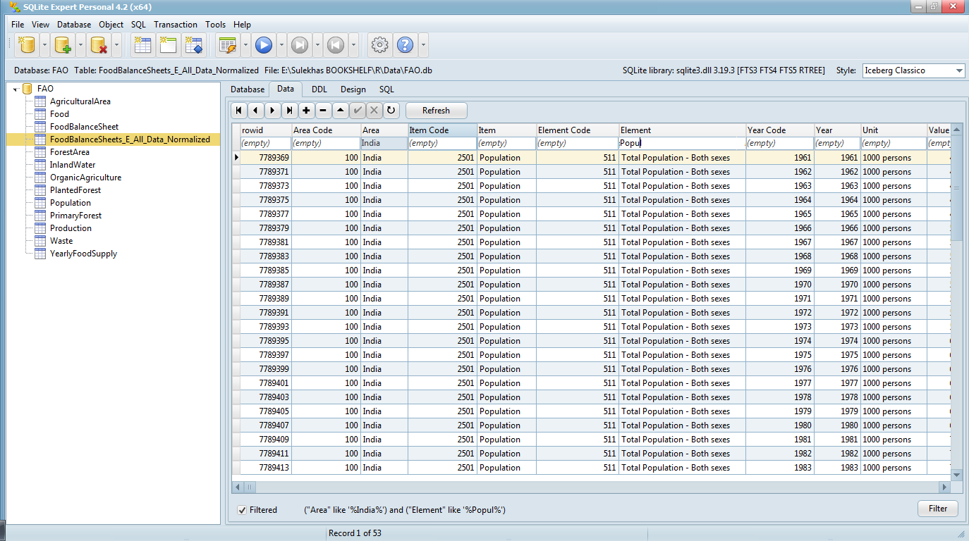
Refined csv data 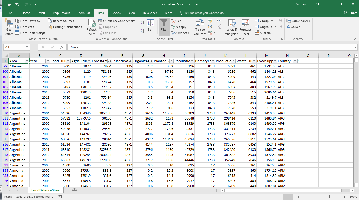
Transform
Data is now transformed in R in such a way that it can be used for exploring, modelling and communicating insights through a dashboard.
R code is divided into two parts:
- Server.R
- UI.R
Further acquiring, refining, transforming, exploring, modelling and communicating are performed within the R code.
*** Dependencies required
require(d3heatmap)
require(dygraphs)
require(xts)
require(ggplot2)
require(plotly)
require(shiny)
require(data.table)
require(forecast)
require(d3scatter)
require(crosstalk)
require(rgl)
require(shinythemes)
Fetch and Transform data
fb <- data.frame(fread("data/FoodBalanceSheet.csv",stringsAsFactors = FALSE))
fb$Year <- as.character(fb$Year)
fb$Year <- paste(fb$Year,"12-31",sep="-")
fb$Year <- as.Date(fb$Year)
fcy <- c("2014-12-31","2015-12-31","2016-12-31","2017-12-31","2018-12-31","2019-12-31",
         "2020-12-31","2021-12-31","2022-12-31","2023-12-31")
fcy <-as.Date(fcy)
fb2<-xts(fb,fb$Year)
Area <- unique(fb$Area)
Date <- as.character(unique(fb$Year))
Create Dashboard UI
UI is created as a multipage (four pages) shiny dashboard with:
- Tab panels
- Sidebar panels
- Selection drop downs
- Help Text
- Interactive charts
- Crosstalk - scatter, bar and rose plots
- Three dimensional cube - RGL Widget
- Heatmap
- Time series charts
- Candel chart
Note: Complete source code is available in Appendix section
sample UI code
shinyUI(
navbarPage("Sulekha Aloorravi - Food & Agriculture Org",
theme = shinytheme("flatly"),
# shinythemes::themeSelector(),
tabPanel("Heatmap",
sidebarPanel(width=2,
selectInput("area", label = "Select Country",
choices = c(Area),
selected = "India"),
selectInput("startdate", label = "Start Date",
choices = c(Date),
selected = "2000-12-31"),
selectInput("enddate", label = "End Date",
choices = c(Date),
selected = "2010-12-31"),
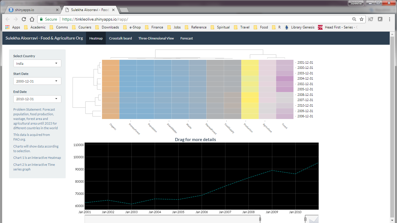
helpText("Problem Statement: Forecast population, food production, wastage, forest area and agricultural area until 2023 for different countries in the world"),
helpText("This data is acquired from FAO.org."),
helpText("Charts will show data according to selection."),
helpText("Chart 1 is an interactive Heatmap"),
helpText("Chart 2 is an interactive Time series graph")
),
mainPanel(
d3heatmapOutput("heat",width="100%",height = "400px"),
dygraphOutput("parallel",width="100%",height = "400px")
)
)))
sample Server code
shinyServer(
function(input, output, session)
{
  cty <- reactive(quote(input$area),quoted=TRUE)
  stdate <- reactive(quote(input$startdate),quoted=TRUE)
  edate<- reactive(quote(input$enddate),quoted=TRUE)
  dates <- reactive({daterow<-fb[which(fb$Area==input$area & fb$Year >= input$startdate & fb$Year<=     input$enddate),2]
  daterow<-as.character(daterow)
  daterow
  })
  sortdt<-reactive(
    {
      heatdata<- fb[which(fb$Area==input$area & fb$Year >= input$startdate & fb$Year<= input$enddate),3:13]
      heatdata
    }
  )

  output$heat<-renderD3heatmap({
    d3heatmap(sortdt(), scale = "row" , colors="Set3",cexRow = 0.8,cexCol = 1,labCol=c

("Agriculture","Organic","FoodSupply","PlantedForest","PrimaryForest","InlandWater","Forest","Waste","Production","FoodSupply","Population"),labRow= dates())
  })

  output$parallel<-renderDygraph(
    dygraph(fb2[fb2$Area==cty(),12], main = "Drag for more details") %>%
      dyRangeSelector(dateWindow = c(stdate(),edate())) %>%
      dySeries(strokeWidth = 2, strokePattern = "dashed") %>%
      dyShading(from = stdate(), to = edate(), color = "black")

  )
})
Explore
Graphs as mentioned in the above section were created to explore data interactively. Shiny dashboard for the same is as follows:
1. Heatmap Tab:
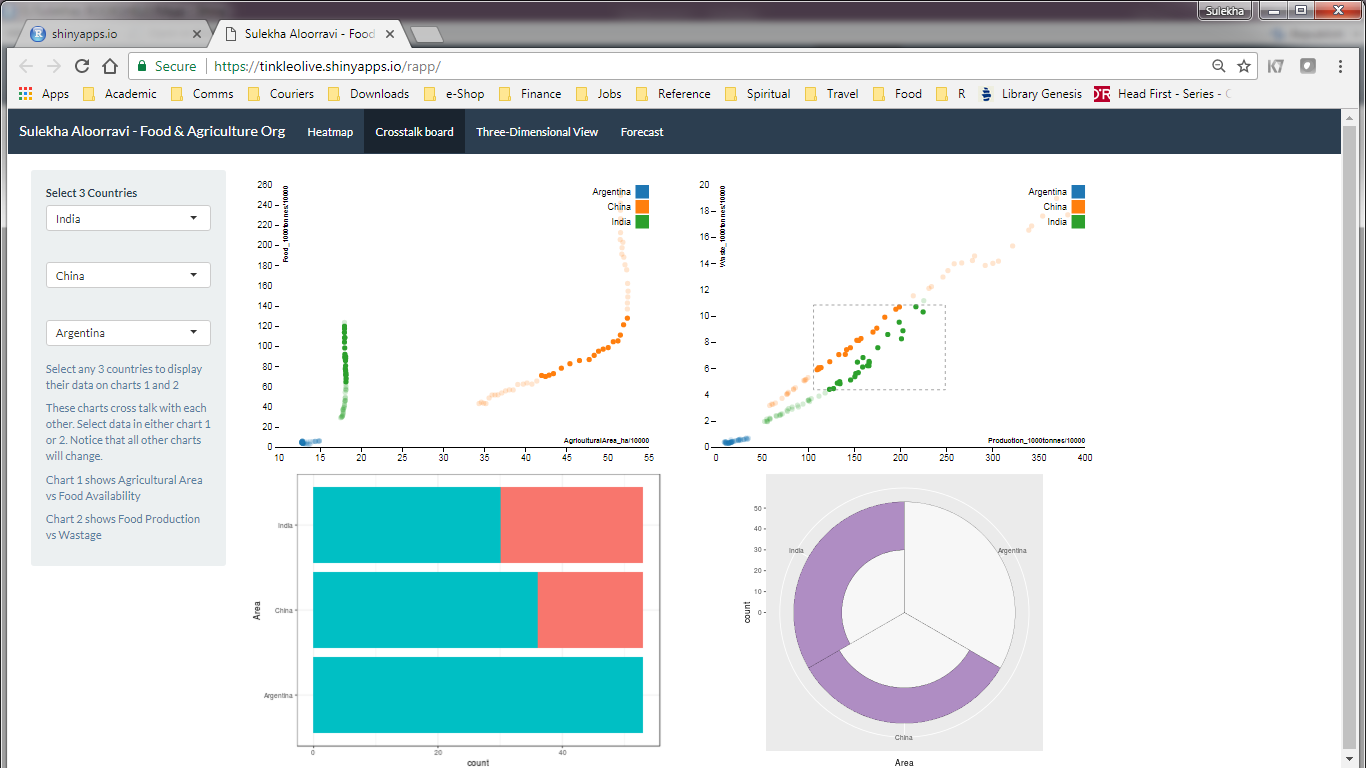
2. Crosstalk Tab:
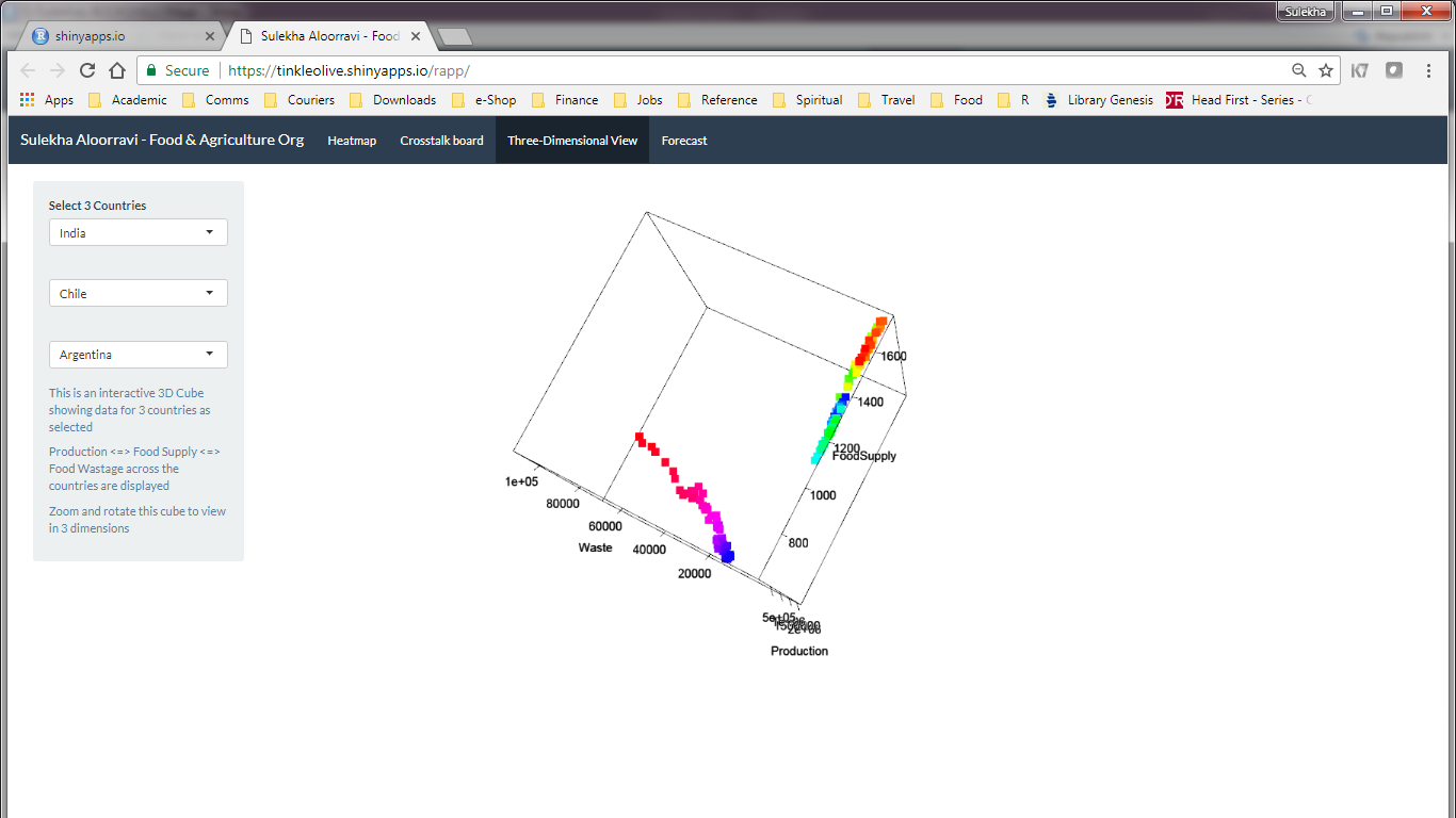
3. Three-dimensional View Tab:
Model
Forecasting of data is performed using ARIMA model.
Explanation: Autoregressice integrated movind average model is fitted to time series to predict future points in the series.
-
In this model, evolving variable of interest is regressed on its own lagged values.
-
Regression error here, is a linear combination of error terms whose values occurred contemporaneously and at various times in the past.
-
The data values have been replaced with the difference between their values and the previous values.
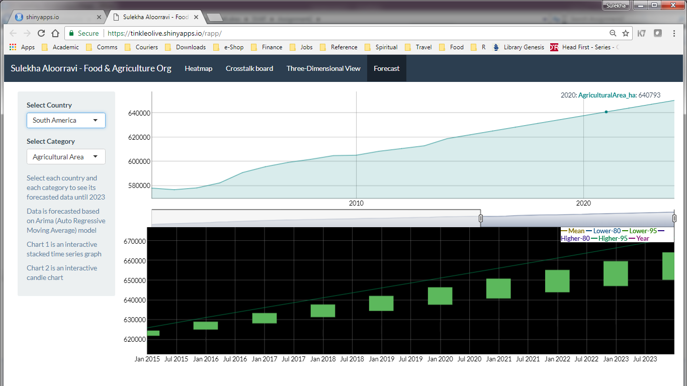
Communicate Insight
From the below charts, trends of Earth’s forecasted data until 2023 are as follows: –Select any country–
-
Agricultural area is becoming less in some countries where as it is increasing in other countries.
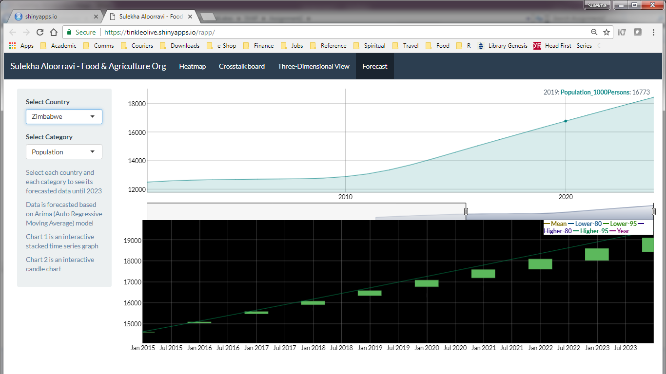
-
Population trend in various countries seem to be uniformly increasing.
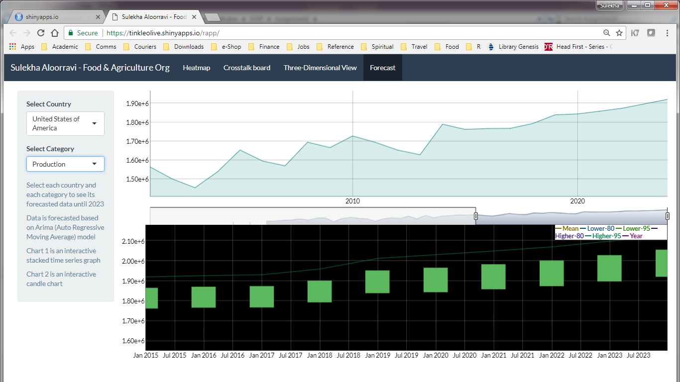
-
Production of food seems to be uniformly increasing.
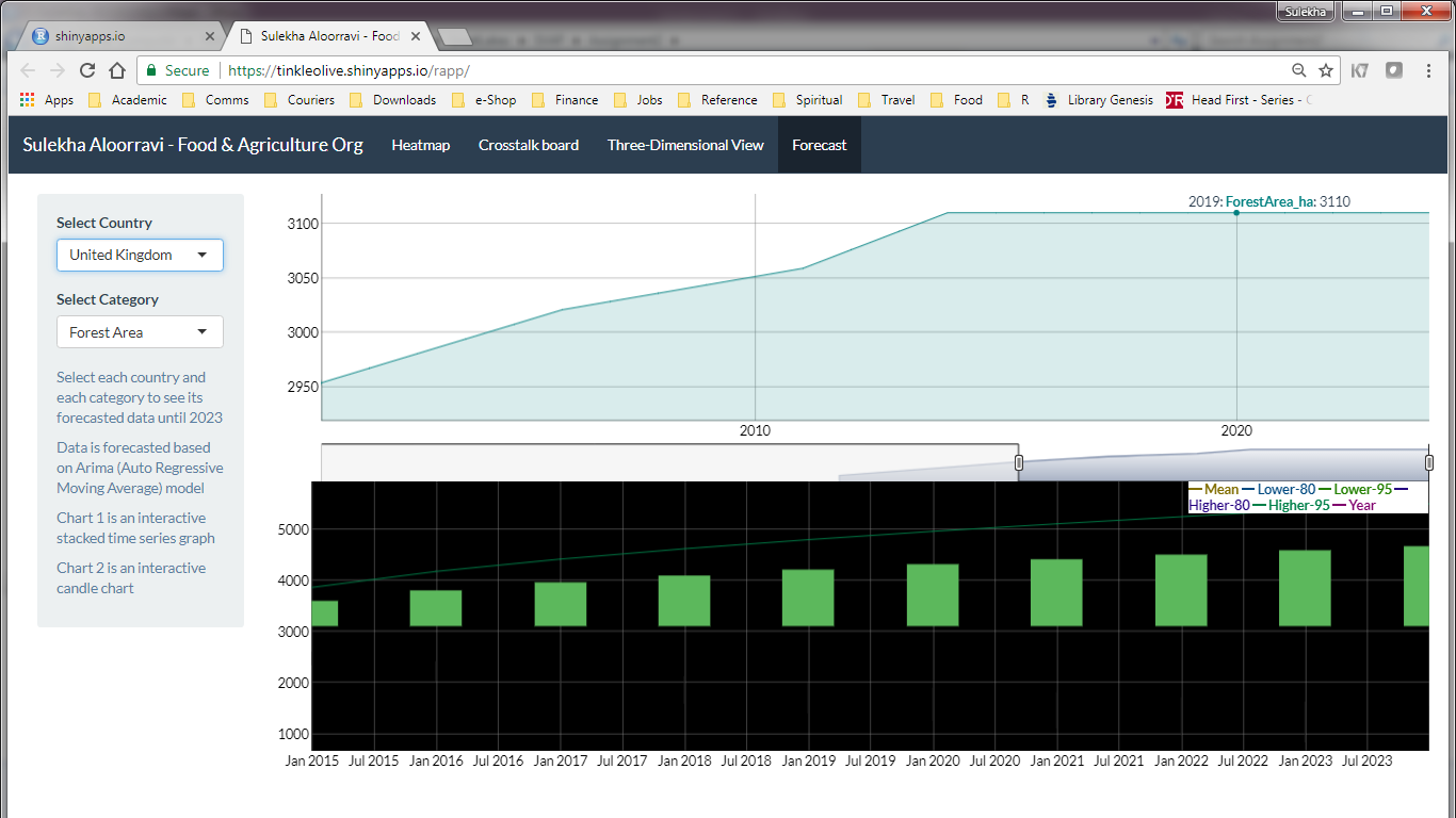
-
Forest either seems to be decreasing or remaining stable in various countries but no evident increase.
-
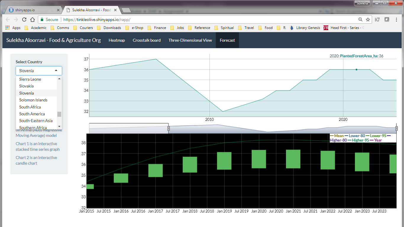
There is no significant increase in planted forest across the world.
-
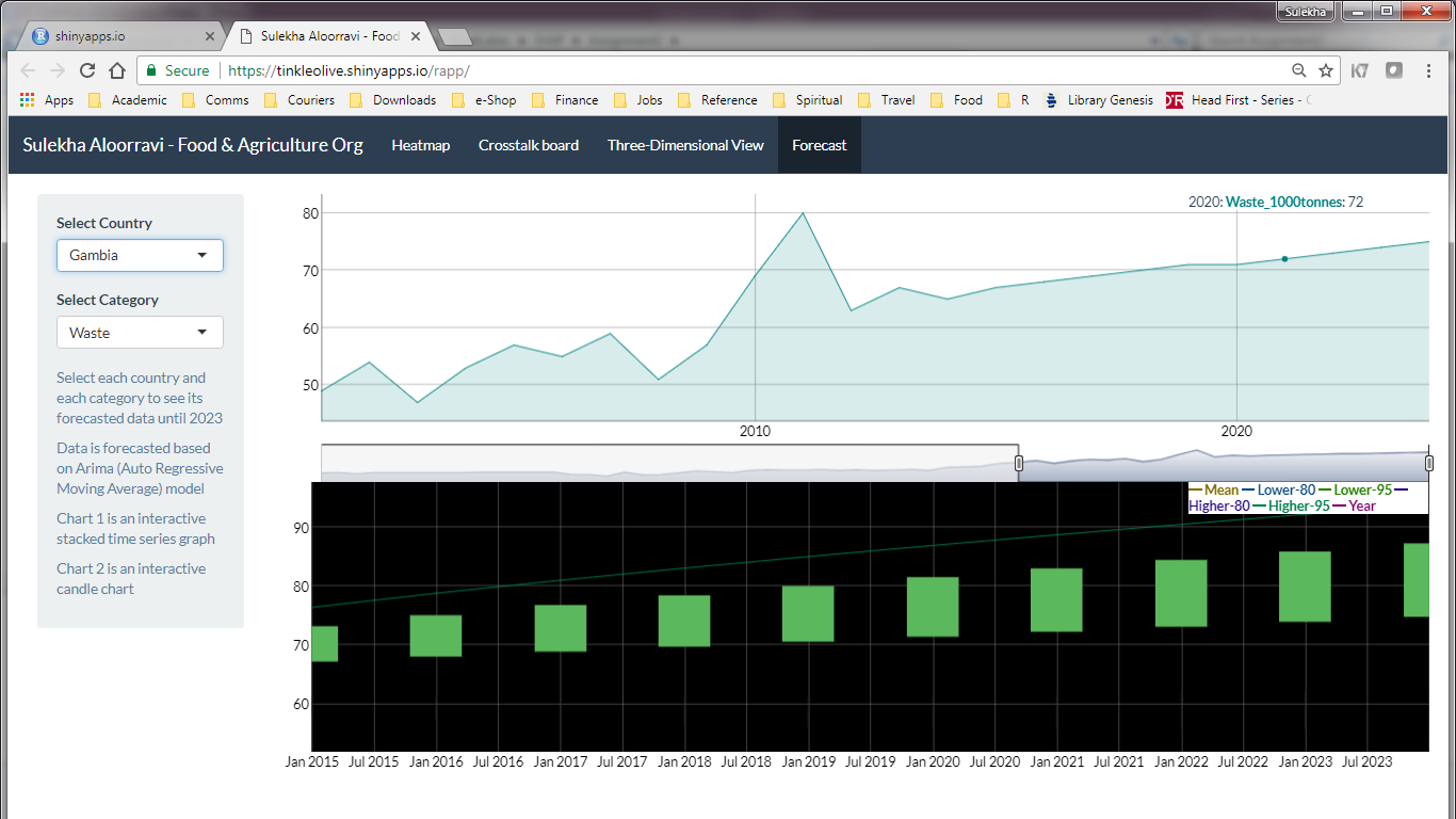
Food wasted across the world is following a stable trend in parallel to the production.
Appendix
UI.R
require(d3heatmap)
require(dygraphs)
require(xts)
require(ggplot2)
require(plotly)
require(shiny)
require(data.table)
require(forecast)
require(d3scatter)
require(crosstalk)
require(rgl)
require(shinythemes)
fb <- data.frame(fread("data/FoodBalanceSheet.csv",stringsAsFactors = FALSE))
fb$Year <- as.character(fb$Year)
fb$Year <- paste(fb$Year,"12-31",sep="-")
fb$Year <- as.Date(fb$Year)
fcy <- c("2014-12-31","2015-12-31","2016-12-31","2017-12-31","2018-12-31","2019-12-31",
"2020-12-31","2021-12-31","2022-12-31","2023-12-31")
fcy <-as.Date(fcy)
fb2<-xts(fb,fb$Year)
Area <- unique(fb$Area)
Date <- as.character(unique(fb$Year))
shinyUI(
navbarPage("Sulekha Aloorravi - Food & Agriculture Org",theme = shinytheme("flatly"),
tabPanel("Heatmap", sidebarPanel(width=2,
selectInput("area", label = "Select Country",choices = c(Area),selected = "India"),
selectInput("startdate", label = "Start Date",choices = c(Date),selected = "2000-12-31"),
selectInput("enddate", label = "End Date", choices = c(Date), selected = "2010-12-31"),
helpText("Problem Statement: Forecast population, food production, wastage, forest area and agricultural area until 2023 for different countries in the world"),
helpText("This data is acquired from FAO.org."),
helpText("Charts will show data according to selection."),
helpText("Chart 1 is an interactive Heatmap"),
helpText("Chart 2 is an interactive Time series graph")
),
mainPanel(
d3heatmapOutput("heat",width="100%",height = "400px"),
dygraphOutput("parallel",width="100%",height = "400px")
)
),
tabPanel("Crosstalk board",
sidebarPanel(width=2,
selectInput("ct1", label = "Select 3 Countries",choices = c(Area),selected = "India"),
selectInput("ct2", label = "", choices = c(Area), selected = "China"),
selectInput("ct3", label = "", choices = c(Area), selected = "Argentina"),
helpText("Select any 3 countries to display their data on charts 1 and 2"),
helpText("These charts cross talk with each other. Select data in either chart 1 or 2. Notice that all other charts will change."),
helpText("Chart 1 shows Agricultural Area vs Food Availability"),
helpText("Chart 2 shows Food Production vs Wastage")
),
mainPanel(
fluidRow(
column(6,
d3scatterOutput("d3sc1")),
column(6,
d3scatterOutput("d3sc2"))
),
fluidRow(
column(6,
plotOutput("cross1")),
column(6,
plotOutput("cross2"))
))
),
tabPanel("Three-Dimensional View",
sidebarPanel(width=2,
selectInput("ca1", label = "Select 3 Countries", choices = c(Area), selected = "India"),
selectInput("ca2", label = "", choices = c(Area), selected = "China"),
selectInput("ca3", label = "", choices = c(Area), selected = "Argentina"),
helpText("This is an interactive 3D Cube showing data for 3 countries as selected"),
helpText("Production <=> Food Supply <=> Food Wastage across the countries are displayed"),
helpText("Zoom and rotate this cube to view in 3 dimensions")
),
mainPanel(
rglwidgetOutput("rgl",width="100%",height="600px")
)),
tabPanel("Forecast",
sidebarPanel(width=2,
selectInput("areafc", label = "Select Country", choices = c(Area), selected = "India"),
selectInput("selectionfc", label = "Select Category", choices = c("Population","Food Availability","Agricultural Area", "Forest Area", "Inland Water Area",
"Organic Farming", "Planted Forest", "Production", "Waste", "Food Supply per Capita"), selected = "Agricultural Area"),
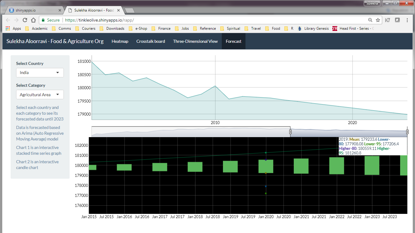
helpText("Select each country and each category to see its forecasted data until 2023"),
helpText("Data is forecasted based on Arima (Auto Regressive Moving Average) model"),
helpText("Chart 1 is an interactive stacked time series graph"),
helpText("Chart 2 is an interactive candle chart")),
mainPanel(width=10,
fluidRow(dygraphOutput("fcdy",width = "100%", height = "300px"),
dygraphOutput("fcdycnd",width="100%",height="300px")))))
)
Server.R
# load data in 'global' chunk so it can be shared by all users of the dashboard
require(data.table)
require(plotly)
require(forecast)
require(d3scatter)
require(crosstalk)

fb <- data.frame(fread("data/FoodBalanceSheet.csv",stringsAsFactors = FALSE))
fb$Year <- as.character(fb$Year)
fb$Year <- paste(fb$Year,"12-31",sep="-")
fb$Year <- as.Date(fb$Year)
fcy <- c("2014-12-31","2015-12-31","2016-12-31","2017-12-31","2018-12-31","2019-12-31",
         "2020-12-31","2021-12-31","2022-12-31","2023-12-31")
fcy <-as.Date(fcy)
fb2<-xts(fb,fb$Year)
Area <- unique(fb$Area)
Date <- as.character(unique(fb$Year))

shinyServer(
function(input, output, session)
{
  cty <- reactive(quote(input$area),quoted=TRUE)
  stdate <- reactive(quote(input$startdate),quoted=TRUE)
  edate<- reactive(quote(input$enddate),quoted=TRUE)
  dates <- reactive({daterow<-fb[which(fb$Area==input$area & fb$Year >= input$startdate & fb$Year<= input$enddate),2]
  daterow<-as.character(daterow)
  daterow
  })
  sortdt<-reactive(
    {
      heatdata<- fb[which(fb$Area==input$area & fb$Year >= input$startdate & fb$Year<= input$enddate),3:13]
      heatdata
    }
  )
  output$heat<-renderD3heatmap({
  d3heatmap(sortdt(), scale = "row" , colors="Set3",cexRow = 0.8,cexCol = 1,labCol=c

("Agriculture","Organic","FoodSupply","PlantedForest","PrimaryForest","InlandWater","Forest","Waste","Production","FoodSupply","Population"),labRow= dates())
  })
  output$parallel<-renderDygraph(
  dygraph(fb2[fb2$Area==cty(),12], main = "Drag for more details") %>%
  dyRangeSelector(dateWindow = c(stdate(),edate())) %>%
  dySeries(strokeWidth = 2, strokePattern = "dashed") %>%
  dyShading(from = stdate(), to = edate(), color = "black")
  )

  d3d<-reactive({
  d3data<-subset(fb,Area == input$ca1 | Area == input$ca2 | Area == input$ca3)
  d3data$Area <-as.factor(d3data$Area)
  d3data
  }
  )

  output$rgl<-renderRglwidget(
      {
      save <- getOption("rgl.useNULL")
      options(rgl.useNULL=TRUE)
      plot3d(x=d3d()[,11],y=d3d()[,12],z=d3d()[,13],xlab="Production",ylab="Waste",zlab="FoodSupply",col=rainbow(nrow(d3d())),size=10,grid=TRUE)
      rglwidget()
    })
  arfc<-reactive(
    {
      region <- subset(fb,Area ==input$areafc)
      if(input$selectionfc == "Population")
      {
        y<-ts(region$Population_1000Persons,frequency = 1)
        fit<-auto.arima(y)
        fc<-forecast(fit, 10)
        meanfc=round(fc$mean)
        pop <- data.frame(cbind(input$areafc,as.character(fcy),meanfc))
        colnames(pop) <- c(colnames(region[,c(1,2,9)]))
        pop$Area <- as.character(pop$Area)
        pop$Year <- as.character(pop$Year)
        pop$Year <- as.Date(pop$Year)
        pop$Population_1000Persons<-as.character(pop$Population_1000Persons)
        pop$Population_1000Persons<-as.numeric(pop$Population_1000Persons)
        fcpop<-rbind(region[,c(1,2,9)],pop)
        fcpop
      }
      else if(input$selectionfc == "Food Availability")
      {
        y<-ts(region$Food_1000tonnes,frequency = 1)
        fit<-auto.arima(y)
        fc<-forecast(fit, 10)
        meanfc=round(fc$mean)
        pop <- data.frame(cbind(input$areafc,as.character(fcy),meanfc))
        colnames(pop) <- c(colnames(region[,c(1,2,3)]))
        pop$Area <- as.character(pop$Area)
        pop$Year <- as.character(pop$Year)
        pop$Year <- as.Date(pop$Year)
        pop$Food_1000tonnes<-as.character(pop$Food_1000tonnes)
        pop$Food_1000tonnes<-as.numeric(pop$Food_1000tonnes)
        fcpop<-rbind(region[,c(1,2,3)],pop)
        fcpop

      }
      else if(input$selectionfc == "Agricultural Area")
      {

        y<-ts(region$AgriculturalArea_ha,frequency = 1)
        fit<-auto.arima(y)
        fc<-forecast(fit, 10)
        meanfc=round(fc$mean)
        pop <- data.frame(cbind(input$areafc,as.character(fcy),meanfc))
        colnames(pop) <- c(colnames(region[,c(1,2,4)]))
        pop$Area <- as.character(pop$Area)
        pop$Year <- as.character(pop$Year)
        pop$Year <- as.Date(pop$Year)
        pop$AgriculturalArea_ha<-as.character(pop$AgriculturalArea_ha)
        pop$AgriculturalArea_ha<-as.numeric(pop$AgriculturalArea_ha)
        fcpop<-rbind(region[,c(1,2,4)],pop)
        fcpop

      }
      else if(input$selectionfc == "Forest Area")
      {

        y<-ts(region$ForestArea_ha,frequency = 1)
        fit<-auto.arima(y)
        fc<-forecast(fit, 10)
        meanfc=round(fc$mean)
        pop <- data.frame(cbind(input$areafc,as.character(fcy),meanfc))
        colnames(pop) <- c(colnames(region[,c(1,2,5)]))
        pop$Area <- as.character(pop$Area)
        pop$Year <- as.character(pop$Year)
        pop$Year <- as.Date(pop$Year)
        pop$ForestArea_ha<-as.character(pop$ForestArea_ha)
        pop$ForestArea_ha<-as.numeric(pop$ForestArea_ha)
        fcpop<-rbind(region[,c(1,2,5)],pop)
        fcpop

      }

      else if(input$selectionfc == "Inland Water Area")
      {

        y<-ts(region$InlandWaterArea_ha,frequency = 1)
        fit<-auto.arima(y)
        fc<-forecast(fit, 10)
        meanfc=round(fc$mean)
        pop <- data.frame(cbind(input$areafc,as.character(fcy),meanfc))
        colnames(pop) <- c(colnames(region[,c(1,2,6)]))
        pop$Area <- as.character(pop$Area)
        pop$Year <- as.character(pop$Year)
        pop$Year <- as.Date(pop$Year)
        pop$InlandWaterArea_ha<-as.character(pop$InlandWaterArea_ha)
        pop$InlandWaterArea_ha<-as.numeric(pop$InlandWaterArea_ha)
        fcpop<-rbind(region[,c(1,2,6)],pop)
        fcpop

      }
      else if(input$selectionfc == "Organic Farming")
      {

        y<-ts(region$OrganicAgricultureArea_ha,frequency = 1)
        fit<-auto.arima(y)
        fc<-forecast(fit, 10)
        meanfc=round(fc$mean)
        pop <- data.frame(cbind(input$areafc,as.character(fcy),meanfc))
        colnames(pop) <- c(colnames(region[,c(1,2,7)]))
        pop$Area <- as.character(pop$Area)
        pop$Year <- as.character(pop$Year)
        pop$Year <- as.Date(pop$Year)
        pop$OrganicAgricultureArea_ha<-as.character(pop$OrganicAgricultureArea_ha)
        pop$OrganicAgricultureArea_ha<-as.numeric(pop$OrganicAgricultureArea_ha)
        fcpop<-rbind(region[,c(1,2,7)],pop)
        fcpop

      }
      else if(input$selectionfc == "Planted Forest")
      {

        y<-ts(region$PlantedForestArea_ha,frequency = 1)
        fit<-auto.arima(y)
        fc<-forecast(fit, 10)
        meanfc=round(fc$mean)
        pop <- data.frame(cbind(input$areafc,as.character(fcy),meanfc))
        colnames(pop) <- c(colnames(region[,c(1,2,8)]))
        pop$Area <- as.character(pop$Area)
        pop$Year <- as.character(pop$Year)
        pop$Year <- as.Date(pop$Year)
        pop$PlantedForestArea_ha<-as.character(pop$PlantedForestArea_ha)
        pop$PlantedForestArea_ha<-as.numeric(pop$PlantedForestArea_ha)
        fcpop<-rbind(region[,c(1,2,8)],pop)
        fcpop

      }
      else if(input$selectionfc == "Production")
      {

        y<-ts(region$Production_1000tonnes,frequency = 1)
        fit<-auto.arima(y)
        fc<-forecast(fit, 10)
        meanfc=round(fc$mean)
        pop <- data.frame(cbind(input$areafc,as.character(fcy),meanfc))
        colnames(pop) <- c(colnames(region[,c(1,2,11)]))
        pop$Area <- as.character(pop$Area)
        pop$Year <- as.character(pop$Year)
        pop$Year <- as.Date(pop$Year)
        pop$Production_1000tonnes<-as.character(pop$Production_1000tonnes)
        pop$Production_1000tonnes<-as.numeric(pop$Production_1000tonnes)
        fcpop<-rbind(region[,c(1,2,11)],pop)
        fcpop

      }

      else if(input$selectionfc == "Waste")
      {

        y<-ts(region$Waste_1000tonnes,frequency = 1)
        fit<-auto.arima(y)
        fc<-forecast(fit, 10)
        meanfc=round(fc$mean)
        pop <- data.frame(cbind(input$areafc,as.character(fcy),meanfc))
        colnames(pop) <- c(colnames(region[,c(1,2,12)]))
        pop$Area <- as.character(pop$Area)
        pop$Year <- as.character(pop$Year)
        pop$Year <- as.Date(pop$Year)
        pop$Waste_1000tonnes<-as.character(pop$Waste_1000tonnes)
        pop$Waste_1000tonnes<-as.numeric(pop$Waste_1000tonnes)
        fcpop<-rbind(region[,c(1,2,12)],pop)
        fcpop

      }

      else if(input$selectionfc == "Food Supply per Capita")
      {

        y<-ts(region$FoodSupply_inKgperCapitaperYear,frequency = 1)
        fit<-auto.arima(y)
        fc<-forecast(fit, 10)
        meanfc=round(fc$mean)
        pop <- data.frame(cbind(input$areafc,as.character(fcy),meanfc))
        colnames(pop) <- c(colnames(region[,c(1,2,13)]))
        pop$Area <- as.character(pop$Area)
        pop$Year <- as.character(pop$Year)
        pop$Year <- as.Date(pop$Year)
        pop$FoodSupply_inKgperCapitaperYear<-as.character(pop$FoodSupply_inKgperCapitaperYear)
        pop$FoodSupply_inKgperCapitaperYear<-as.numeric(pop$FoodSupply_inKgperCapitaperYear)
        fcpop<-rbind(region[,c(1,2,13)],pop)
        fcpop

      }
      fcfb<-xts(fcpop,fcpop$Year)
    }

  )

  arfcand<-reactive(

    {
      region1 <- subset(fb,Area ==input$areafc)
      if(input$selectionfc == "Population")
      {
        y1<-ts(region1$Population_1000Persons,frequency = 1)
        fit1<-auto.arima(y1)
        fc1<-forecast(fit1, 10)
        fccand<-data.frame(cbind(fc1$mean,fc1$lower,fc1$upper,as.character(fcy)))
        colnames(fccand)<-c("Mean","Lower-80","Lower-95","Higher-80","Higher-95","Year")
        fccand$Year <- as.character(fccand$Year)
        fccand$Year <- as.Date(fccand$Year)
      }
      else if(input$selectionfc == "Food Availability")
      {

        y1<-ts(region1$Food_1000tonnes,frequency = 1)
        fit1<-auto.arima(y1)
        fc1<-forecast(fit1, 10)
        fccand<-data.frame(cbind(fc1$mean,fc1$lower,fc1$upper,as.character(fcy)))
        colnames(fccand)<-c("Mean","Lower-80","Lower-95","Higher-80","Higher-95","Year")
        fccand$Year <- as.character(fccand$Year)
        fccand$Year <- as.Date(fccand$Year)

      }
      else if(input$selectionfc == "Agricultural Area")
      {

        y1<-ts(region1$AgriculturalArea_ha,frequency = 1)
        fit1<-auto.arima(y1)
        fc1<-forecast(fit1, 10)
        fccand<-data.frame(cbind(fc1$mean,fc1$lower,fc1$upper,as.character(fcy)))
        colnames(fccand)<-c("Mean","Lower-80","Lower-95","Higher-80","Higher-95","Year")
        fccand$Year <- as.character(fccand$Year)
        fccand$Year <- as.Date(fccand$Year)

      }
      else if(input$selectionfc == "Forest Area")
      {

        y1<-ts(region1$ForestArea_ha,frequency = 1)
        fit1<-auto.arima(y1)
        fc1<-forecast(fit1, 10)
        fccand<-data.frame(cbind(fc1$mean,fc1$lower,fc1$upper,as.character(fcy)))
        colnames(fccand)<-c("Mean","Lower-80","Lower-95","Higher-80","Higher-95","Year")
        fccand$Year <- as.character(fccand$Year)
        fccand$Year <- as.Date(fccand$Year)

      }

      else if(input$selectionfc == "Inland Water Area")
      {

        y1<-ts(region1$InlandWaterArea_ha,frequency = 1)
        fit1<-auto.arima(y1)
        fc1<-forecast(fit1, 10)
        fccand<-data.frame(cbind(fc1$mean,fc1$lower,fc1$upper,as.character(fcy)))
        colnames(fccand)<-c("Mean","Lower-80","Lower-95","Higher-80","Higher-95","Year")
        fccand$Year <- as.character(fccand$Year)
        fccand$Year <- as.Date(fccand$Year)

      }
      else if(input$selectionfc == "Organic Farming")
      {

        y1<-ts(region1$OrganicAgricultureArea_ha,frequency = 1)
        fit1<-auto.arima(y1)
        fc1<-forecast(fit1, 10)
        fccand<-data.frame(cbind(fc1$mean,fc1$lower,fc1$upper,as.character(fcy)))
        colnames(fccand)<-c("Mean","Lower-80","Lower-95","Higher-80","Higher-95","Year")
        fccand$Year <- as.character(fccand$Year)
        fccand$Year <- as.Date(fccand$Year)

      }
      else if(input$selectionfc == "Planted Forest")
      {

        y1<-ts(region1$PlantedForestArea_ha,frequency = 1)
        fit1<-auto.arima(y1)
        fc1<-forecast(fit1, 10)
        fccand<-data.frame(cbind(fc1$mean,fc1$lower,fc1$upper,as.character(fcy)))
        colnames(fccand)<-c("Mean","Lower-80","Lower-95","Higher-80","Higher-95","Year")
        fccand$Year <- as.character(fccand$Year)
        fccand$Year <- as.Date(fccand$Year)

      }
      else if(input$selectionfc == "Production")
      {

        y1<-ts(region1$Production_1000tonnes,frequency = 1)
        fit1<-auto.arima(y1)
        fc1<-forecast(fit1, 10)
        fccand<-data.frame(cbind(fc1$mean,fc1$lower,fc1$upper,as.character(fcy)))
        colnames(fccand)<-c("Mean","Lower-80","Lower-95","Higher-80","Higher-95","Year")
        fccand$Year <- as.character(fccand$Year)
        fccand$Year <- as.Date(fccand$Year)

      }

      else if(input$selectionfc == "Waste")
      {

        y1<-ts(region1$Waste_1000tonnes,frequency = 1)
        fit1<-auto.arima(y1)
        fc1<-forecast(fit1, 10)
        fccand<-data.frame(cbind(fc1$mean,fc1$lower,fc1$upper,as.character(fcy)))
        colnames(fccand)<-c("Mean","Lower-80","Lower-95","Higher-80","Higher-95","Year")
        fccand$Year <- as.character(fccand$Year)
        fccand$Year <- as.Date(fccand$Year)

      }

      else if(input$selectionfc == "Food Supply per Capita")
      {

        y1<-ts(region1$FoodSupply_inKgperCapitaperYear,frequency = 1)
        fit1<-auto.arima(y1)
        fc1<-forecast(fit1, 10)
        fccand<-data.frame(cbind(fc1$mean,fc1$lower,fc1$upper,as.character(fcy)))
        colnames(fccand)<-c("Mean","Lower-80","Lower-95","Higher-80","Higher-95","Year")
        fccand$Year <- as.character(fccand$Year)
        fccand$Year <- as.Date(fccand$Year)

      }
      cand<-xts(fccand,fccand$Year)
    }

  )

  selfc <- reactive(quote(input$selectionfc),quoted=TRUE)

  output$fcdy<-renderDygraph(
        dygraph(arfc()[,3]) %>%
      dyRangeSelector(dateWindow = c("2000-12-31","2023-12-31")) %>%
      dyOptions(stackedGraph = TRUE)
  )
  output$fcdycnd<-renderDygraph(
    dygraph(arfcand()) %>%
     dyCandlestick() %>%
      dyShading(from="2013-12-31",to="2023-12-31",color = "black")
  )
  crs<-reactive(
    {
      fbcross<-subset(fb,Area == input$ct1 | Area == input$ct2 | Area == input$ct3 )
      shared_fb<-SharedData$new(fbcross)
      shared_fb
    })
  output$d3sc1<-renderD3scatter({
     d3scatter(crs(), ~AgriculturalArea_ha/10000, ~Food_1000tonnes/10000, ~Area, width = "100%")
    })

  output$d3sc2<-renderD3scatter({
     d3scatter(crs(), ~Production_1000tonnes/10000, ~Waste_1000tonnes/10000, ~Area, width = "100%")
    })
  df <- reactive(crs()$data(withSelection = TRUE))
  output$cross1<-renderPlot({
      ggplot(df(), aes(Area, fill = crosstalk::selection_factor(selected_))) +
      geom_bar(stat = "count") +
      coord_flip() +
      theme_bw() +
     theme(legend.position = 'none')
  })
  output$cross2<-renderPlot({
      ggplot(df(), aes(Area, fill = crosstalk::selection_factor(selected_))) +
      geom_bar(stat = "count",colour="black",width=1,size=0.1) +
      scale_fill_brewer(palette = "PRGn", direction=1) +
      theme(legend.position = 'none')+
      coord_polar()
    })
  })